Introduction¶

Table of Contents:

Basics and Language
Logic and Computation
Language Games
Naming and Necessity
Deep Learning
Large Language Models
Algebraic Topology and Categories
Type Theory
Theorem Proving
Models of the Mind
Scaling RL for LLMs
Compression
Symbolic Reasoning
Strong Trial and Error
Thinking Machines

The purpose of this book is not to convince you of anything or spare you from thinking about the foundation of mathematics, language or computation which have evolved over centuries. Rather it is to give you enough context and rigor that you can start questioning and thinking about these things for yourself.

Now what could be a better place to start introducing you to everything that we want to talk about than a question phrased in the likening of Socrates.

What is a symbol that you and I may know it, what are we that symbols may be known to us, and how may we arrange rocks that they may know a symbol too?

It’s a simple question (inspired from a Warren McCulloch article) but its underbelly forms a fucking Langlands Program.

Does a symbol represent anything (reality / meaning / concepts) beyond its syntax?
- Intentionality, Philosophy of Mind
- Definition Problem, Philosophical Logic
- Internal Representation Problem, Cognitive Science
How does a symbol acquire meaning?
- Grounding Problem, Philosophy of Language
Can we replace symbol for program (in a machine) / proof (in a logic) / path (in a shape)?
- Foundation Problem, Mathematics
- Curry Howard Lambek Correspondence, Computer Science
- Definition Problem, Mathematical Logic
Is knowing not computational?
- Church-Turing Hypothesis, Computer Science
- Weak and Hard Problem of Consciousness, Cognitive Science
What does it mean to know?
- Gettier Problem, Epistemology

Going with our parable of arranging rocks, if there is one thing that I would want you to take away from this book, it is that everything we discuss here is utterly useless if we don't try to build anything out of it and to build anything would be utterly useless if it doesn't free us to do useless things (absurd subjective destitution).

As you read, you'll notice this book is poor in academic jargon and formalism. This is intentional. I've seen too many papers and books prioritize “sophistication” over being genuinely helpful.

Sometimes such sophistication is essential. Especially if you want to do careful maintenance and authoritative referencing. But not when you want to plant a tree rather than tend a garden.

I will try to keep things:

Simple and coherent enough to understand
Rigorous enough to experiment with
Succinct enough to use as a primitive module / concept / abstraction
Interesting enough to actually give a shit

This isn’t just hand-waving. The dynamic between coherence or semantic fidelity with succinctness or compression reflects a fundamental tradeoff in how we learn and understand.

Basics and Language¶

In the beginning, God created “אב”. (Genesis 1:1)

In the beginning God created “naming and asserting definite existence from names—with which he made” the heavens and the earth. An homage to the importance of language and naming.

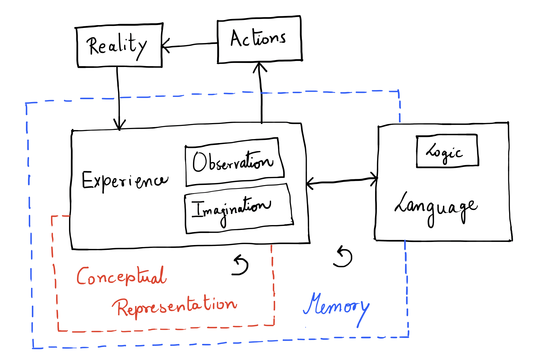
Conceptual Representation¶

Conceptual representation can be (at least):

Compositional
Recursive
Narrative (> strong temporal coherence)
Self-referential
Multi-modal

Thus, the CR space has to be hierarchical by definition. Spanning and binding requirements must exist which can also tell us why some representations are better than others for particular use cases.

Can spanning and binding (SR dynamics) be the base for compression and coherence? Can we think of precision, reliability, efficiency and fidelity just in terms of SR dynamics or do we need more axes?

Planning and reasoning as computational processes?
Is world model an emergent property? If not should it be completely inside CR-space? The argument for world model is satisfying the need to learn representing the world in a non task-specific way.
Any collapsibility criteria?

We mentioned that CR is multimodal. Well, what are some of the modes of operation (ranked in order of abstractness)?

Logical
Spatial
Linguistic
Musical (more to do with timing than hearing)
Emotional (includes interpersonal too, hence lower)
Naturalistic (general observation)
Kinesthetic (movement)

Intelligence¶

What is intelligence and how should we measure it for machines?

If we want to do it in terms of generalization, we need to control experience and priors (already learnt concepts).
Examinations are not a good proxy for measuring intelligence of current machines since these were designed for humans under the latent assumptions that they need to perform generalization to do well. Such latent assumptions do not hold for machines.

Is being conscious necessary to being generally intelligent (probably not)?

Language¶

Stories are how we sense reality. And language serves an approximate communicator of (and about hence recursive) stories.

But words can also utterly confound us. Hop on the wrong ones while playing across language games, and you shall see.

All of language is analogy. Some of those analogies are logical.
To communicate is not the same as to be.
Isn’t all of symbolic representation is language?

Knowledge¶

I know that I know nothing. (Socrates)

Plato said knowledge, classically, is defined as justified true belief. In other words:

\(S\) knows \(P\) if and only if:

\(P\) is true.
\(S\) accepts \(P\).
\(S\) has adequate evidence for \(P\).

But is that sufficient? Well it was thought to be so until in 1963 Edmund Gettier under pressure to publish something submitted a 3 page article to the Analysis journal.

Gettier Problem¶

Suppose: You have asked John about his car multiple times to infer that yep, it is indeed owned by him. And Blake has never been to anywhere outside of Staten Island.

\[ A = \text{John owns a Ford} \]

\[ B = \text{Blake is in Staten Island} \]

\[ \text{Claim:}\quad A, (A \to A\vee B) \vdash A\vee B \]

Now suppose that due to some random event, John doesn’t own a Ford (the bank took it away, they say) but Blake ends up in Staten Island. Then \(P = A \vee B\) is still true. Thus we have that:

\(P\) is true
You have accepted \(P\) to be true.
You are reasonable justification for \(P\) being true.

But did you really know \(P\)?

Meaning¶

[TODO: type out my notes]

Logic and Computation¶

[TODO: type out my notes]

Logic¶

[TODO: logic, object logic, meta logic]

Computation¶

CTD Principle: A (quantum) Turing machine can simulate any physical process.
CTD Thesis: A quantum Turing machine can efficiently (within polynomial overhead — why polynomial? because compositionality) simulate any realistic model of computation.
But what is computation? Any process that transforms information.

Why does the CTD Principle makes sense? Because we assume that most process in the universe follow some form of logic. And Turing machines are just models which can execute such logic.

Interestingly, from this we can also figure out requirements that a Turing machine must satisfy. Namely, being able to execute any condition and doing so again and again indefinitely. It implements:

Conditional branching
Indefinite iteration
Read, write or update operations over symbols
Unbounded storage (let’s not call it memory)

A Turing machine is a 5 tuple. Anything a universal Turing machine can decide on or compute is an algorithm.

\[M = \left(Q, \Gamma, \delta, q_0, h\right)\]

\[\text{where } \Gamma = \Sigma \cup \{\_\}\]

\[\delta: Q \times \Gamma \to Q \times \Gamma \times \{\text{left, right}\}\]

So what are then uncomputable things like? Here is an example.

# Hypothetical HALTS function
def HALTS(program_text, input_data):
    # Somehow magically determines if program_text halts on input_data
    # Returns True if halts, False if runs forever
    pass

# The troublemaker program
def TROUBLE(program_text):
    if HALTS(program_text, program_text):
        # If it halts, loop forever
        while True:
            pass
    else:
            # If it doesn't halt, halt immediately
        return

# Convert TROUBLE to its string representation
trouble_source = get_program_text(TROUBLE)

# What happens here?
# We prove that HALTS cannot exist
TROUBLE(trouble_source)

Language: Set of strings over alphabet \(\Sigma\)
- \(L \subseteq \{0, 1\}^*\) when we fuck everything into binary shit, \(\Sigma\) becomes \(\{0, 1\}\)
- Any mathematical object can be encoded as a binary string.
Decision Problem: Is \(w \in L\)?
- Any problem is a mapping from a set of inputs to a set of outputs.
- Any computational problem can be converted into a decision problem.
  
  \[f:\{0,1\}^*\to \{0,1\}^*\]
  
  \[G(f)=\{(x,y):f(x)=y\}\subseteq\{0,1\}^*\]
- Any function \(f\) can be computed iff its graph \(G(f)\) can be decided.
- TM decides \(L\): \(\forall w\), TM halts, accepts iff \(w \in L\), rejects iff \(w \notin L\).
- A language \(L\) is called decidable if \(\forall w,\ \exists M\) which accepts when \(w \in L\) and rejects otherwise.
- A language \(L\) is called recognizable if when \(w \notin L\), \(M\) doesn’t halt but accepts otherwise.
- A language is called unrecognizable if \(\nexists M\) that recognizes it. Example: complement of the halting problem.
- If \(C\) is a complexity class, it can be defined as follows. Often while defining resource bounds we try to deal with polynomials because they are closed under composition.

\[ C =\{L \subseteq \{0,1\}^*: L \text{ can be decided within resource bound } f(n) \text{ on model } M\} \]

Here is a list of several complexity classes.

Say you have two decision problems \(A\) and \(B\). Then, \(A\) is said to be reducible to \(B\) if \(B\) can be used as a subroutine for \(A\). Then obviously, \(A\) is at most as hard as \(B\ (A\leq B)\) .

Comparing logic systems and their complexities.

Logic System	Intuitive Explanation	Satisfiability	Validity	Model Check
Classical Logic
Propositional Logic	Basic logic with AND, OR, NOT - no quantifiers over variables	NP-c	coNP-c	\(\in P\)
Horn Clauses	Restricted propositional logic where each clause has \(\leq1\) positive literal	P-c	P-c	\(\in P\)
First-Order Logic	Logic with quantifiers \(\exists, \forall\) over individual objects/variables	coRE-c	RE-c	PSPACE-c
Monadic First-Order	First-order logic restricted to unary (single-argument) predicates only	NEXP-c	coNEXP-c	—
Intuitionistic Logic
Propositional	Constructive logic, rejects law of excluded middle, requires explicit proofs	PSPACE-c	PSPACE-c	P-c
First-Order	Constructive first-order logic with explicit existence proofs required	coRE-c	RE-c	—
Modal Logic
\(K, T, S4\)	Necessity (\(\square\)) and possibility (\(\large\diamond\)) with different axioms about accessibility	PSPACE-c	PSPACE-c	P-c
\(S5\)	Modal logic where accessibility relation is equivalence (reflexive, symmetric, transitive)	NP-c	coNP-c	\(\in P\)
Epistemic Logic
\(S5_n (n\geq 2)\)	Multi-agent knowledge logic - what agents know about others' knowledge	PSPACE-c	PSPACE-c	—
\(K_n^C, T_n^C (n\geq2)\)	Epistemic logic with common knowledge operator - what everyone knows that everyone knows	EXP-c	EXP-c	—

What does asking computational complexity of logic systems even mean?

Model checking asks: "Does this model (object values) is this formula satisfied?"
Satisfiability asks: "Does any model (object value assignment) satisfy this formula?"
Validity asks: "Do all material value assignments satisfy this formula?"

Disjunctions¶

Is all thinking computational?

[TODO: type out my notes]

Language Games¶

[TODO: type out my notes]

Naming and Necessity¶

[TODO: type out my notes]

Deep Learning¶

Artificial Intelligence is based on the idea of physical systems which can learn to do (def: solve) stuff.

\[ \text{Stuff:}\quad\text{Puzzles} → \text{Problems} → \text{Class of problems} → \text{Skills} → \text{Processes} \]

Rule based: Conditionals.
Classical Machine Learning: Constrained geometric optimization where you assume predefined geometric structures for the solution and optimize under its constraints.
- Linear and non-linear regression: curve fitting.
- Logistic regression and SVM: separating planes (in SVM you map data into higher dimensions where planar separation works).
- Decision trees and random forests: partitioning space.
- Clustering: similarity grouping in space even hierarchically.
- Naive Bayes: Model probability distributions for each feature (assumes features are independent given the class).
Deep Learning: Adaptive geometric optimization with implicit biases.
- DL biases are more about the learning process (hierarchical feature extraction, reusability of local patterns etc.) and computational structure than solution geometry.
- But then what about graph neural networks and shit?
- Even in GNNs and Geometric DL, the focus is on computational biases that respect geometry (like rotations / translations).
- Why the fuck is “geometry” everywhere? Because geometry is just a good description for spatial relationships.
Reinforcement Learning: trial-and-error and a completely different paradigm.

Neural Networks¶

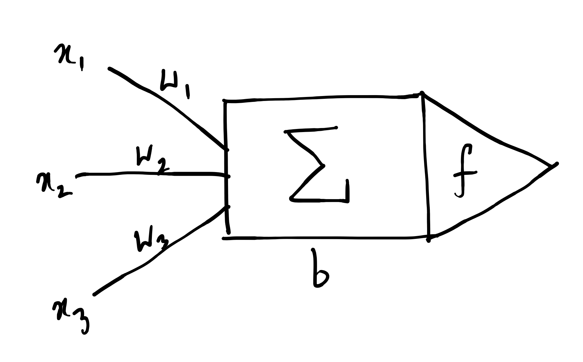
\(\Sigma\) is the transfer function. \(\vec{w} + [b]\) are the parameters.

\(f\) is the non-linear activation function. For example, \(\sigma(\cdot)\) as the sigmoid function.

\[ y= f(\vec w \cdot \vec x + b) = f(\vec z) \]

Some generic notes on deep learning:

The universal neuron is always a vector-to-scalar map.
Layers can be vectors and them being adjacently stacked can lead to tensors.

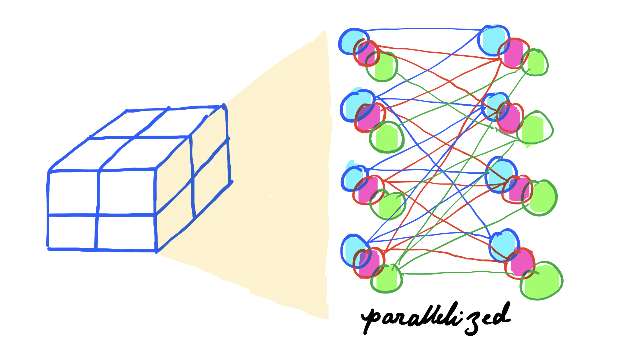
However, we can abstract this into a tensor-to-tensor form through composition of multiple vector-scalar-maps.

Backpropagation¶

Backprop is basically a recursive application of chain rule backwards through the computational graph.

Gradient Descent¶

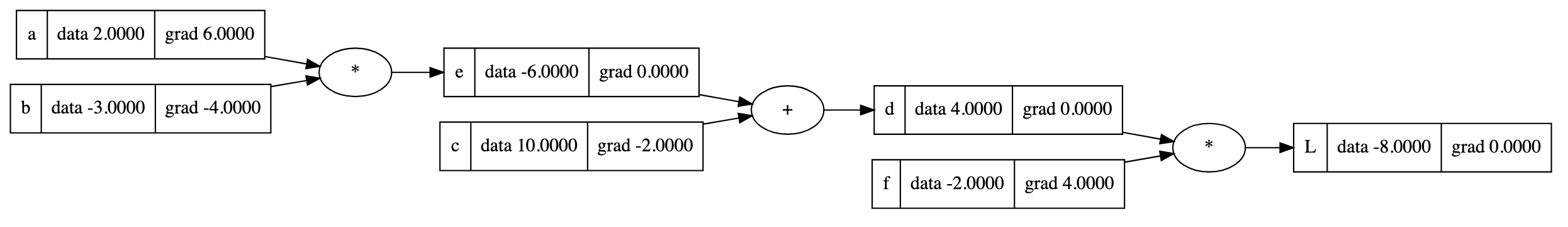
Consider a computational graph representing the function:

\[ L = (a \times b + c) \times f \]

where the intermediate variables are defined as:

\[ e = a \times b,\quad d = e + c = a \times b + c, \quad L = d \times f \]

Suppose the initial values of the variables are \(a_0 = 2\), \(b_0 = -3\), \(c_0 = 10\), \(f_0 = -2\).

\[ L_0 = d_0 \times f_0 = 4 \times (-2) = -8 \]

The gradients are manually assigned (fixed) as

\[ \frac{\partial L}{\partial a} = 6, \quad \frac{\partial L}{\partial b} = -4, \quad \frac{\partial L}{\partial c} = -2, \quad \frac{\partial L}{\partial f} = 4 \]

and assuming a gradient ascent rule with learning rate \(\alpha = 0.01\) thus optimizing \(L\) towards zero using fixed gradient. Hence, we have \(a_n = 2 + 0.06n, b_n = -3 - 0.04n, c_n = 10 - 0.02n, f_n = -2 + 0.04n\).

\[ {L_n = -8 + 0.72n - 0.0064n^2 - 0.000096n^3} \]

Plotting the function here.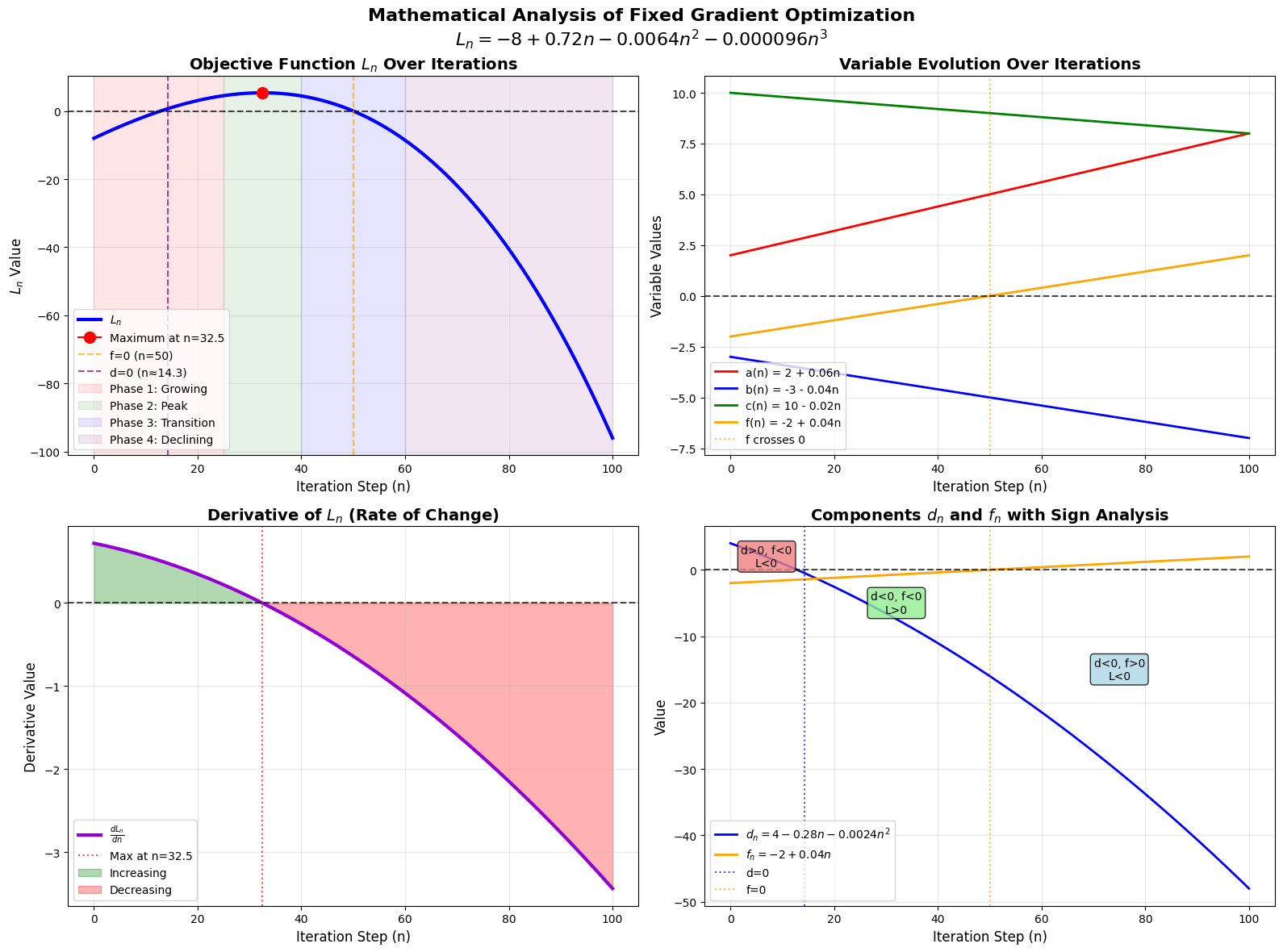

This is half the picture. We have been doing fixed gradient descent and it can overshoot optimal solutions if the gradients don't adapt.

We need to update the parameters themselves. \(\frac{\partial L}{\partial a} = 6 \not\equiv \frac{\partial L}{\partial a} = bf\) and clearly, \(b_0f_0 = 6\) but \(b_1f_1 = 5.96\) and so on. The fixed gradient approach is essentially performing a linear approximation of the loss surface that becomes increasingly inaccurate as you move away from the initial point. We should rather continuously recompute gradients to adapt to the changing curvature of the loss space.

Implementing Backpropagation¶

\[ \text{Value} \to \text{Neuron} \to \text{Layer} \to \text{MLP} \]

Defining a class Value.

import math

class Value:

    def __init__(self, data, parents=(), op="", label = ""):
        self.data: float = data
        self.grad: float = 0
        self.op: str = op
        self.backprop = lambda: None
        self.parents: set = set(parents)
        self.label: str = label

    def __repr__(self):
        return f"Value(data={self.data})"

    def __add__(self, other):
        other = other if isinstance(other, Value) else Value(other)
        out = Value(self.data + other.data, (self, other), "+")

        def backprop():
            self.grad += out.grad * 1.0
            other.grad += out.grad * 1.0

        out.backprop = backprop
        return out

    def __mul__(self, other):
        other = other if isinstance(other, Value) else Value(other)
        out =  Value(self.data * other.data, (self, other), "*")

        def backprop():
            self.grad += out.grad * other.data
            other.grad += out.grad * self.data

        out.backprop = backprop
        return out

    def __radd__(self, other):
        return self + other

    def __rmul__(self, other):
        return self * other

    def __pow__(self, other):
        assert isinstance(other, (int, float)), "int/float powers for now"
        out = Value(self.data**other, (self,), f"**{other}")

        def backprop():
            self.grad += out.grad * other * self.data**(other - 1)

        out.backprop = backprop
        return out

    def __truediv__(self, other):
        return self * other**-1

    def __neg__(self):
        return self * -1

    def __sub__(self, other):
        return self + (-other)

    def exp(self):
        x = self.data
        e = math.exp(x)
        out = Value(e, (self,), "exp")

        def backprop():
            self.grad += out.grad * e

        out.backprop = backprop
        return out

    def tanh(self):
        n = self.data
        t = (math.exp(2*n) - 1)/(math.exp(2*n) + 1)
        out = Value(t, (self,), "tanh")

        def backprop():
            self.grad += out.grad * (1 - t**2)

        out.backprop = backprop
        return out

        def relu(self):
        out = Value(0 if self.data < 0 else self.data, (self,), 'relu')

        def backprop():
            self.grad += (out.data > 0) * out.grad

        out.backprop = backprop
        return out

    def backward(self):
        visited = set()
        def dfs(u):
            u.backprop()
            visited.add(u)
            for v in u.parents:
                if v not in visited:
                    dfs(v)
        self.grad = 1.0
        dfs(self)

Defining a class Neuron.

import random

class Neuron:

    def __init__(self, num_inputs):
        self.w = [Value(random.uniform(-1, 1)) for _ in range(num_inputs)]
        self.b = Value(random.uniform(-1, 1))

    def __call__(self, x):
        act = sum((wi * xi for wi, xi in zip(self.w, x)), self.b)
        out = act.tanh()
        return out

    def parameters(self):
        return self.w + [self.b]

Defining a class Layer.

class Layer:

    def __init__(self, num_inputs, num_outputs):
        self.neurons = [Neuron(num_inputs) for _ in range(num_outputs)]

    def __call__(self, x):
        outs = [n(x) for n in self.neurons]
        return outs[0] if len(outs) == 1 else outs

    def parameters(self):
        return [p for neuron in self.neurons for p in neuron.parameters()]

Defining a class MLP.

class MLP:

    def __init__(self, num_inputs, list_outputs):
      size = [num_inputs] + list_outputs
        self.layers = [Layer(
            size[i], 
            size[i + 1]
        ) for i in range(len(list_outputs))]

  def __call__(self, x):
      for layer in self.layers:
        x = layer(x)
      return x

  def parameters(self):
    return [p for layer in self.layers for p in layer.parameters()]

\[ \text{Forward Pass} \to \text{Loss} \to \text{Backward Pass} \to \text{Update params and grad} \]

Implementing training.

for k in range(num):
    # forward pass
    ypred = [mlp(x) for x in xs]
    losses = [(yout - ygt)**2 for ygt, yout in zip(ys, ypred)]
    loss = sum(losses)

    # backward pass
    loss.backward()

    # update params and grad
    for p in mlp.parameters():
        p.data += -0.05 * p.grad
        p.grad = 0

    print(k, loss.data)

Universal Approximation¶

A bounded depth (1 hidden) and unbounded width shallow neural network is an universal approximator.
- Sigmoid creates stepwise functions (stacking).
  
  \[ \text{Core Idea}:\quad f(x) = \sum \pm\ \text{scale with direction} \cdot \sigma(w(x - \text{position})) \]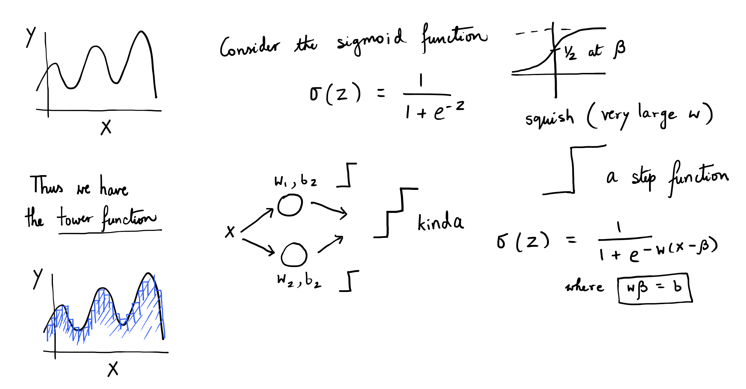
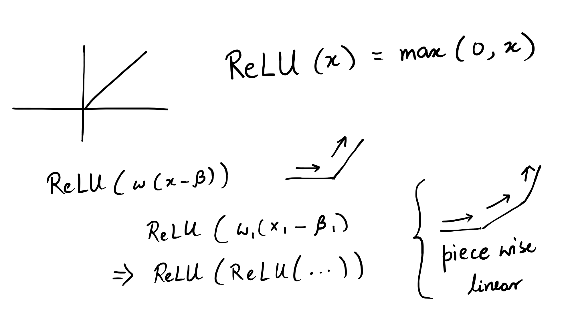
A bounded width (1 per layer) and unbounded depth neural network is an universal approximator.
- ReLU creates piecewise linear functions (composition).
A bounded depth and bounded width (2 of each) NN is a universal approximator.

Hey so isn’t polynomial regression universal approximator too? Well theoretically yes, but they suffer from:

being numerically unstable
oscillate wildly between data points (Runge’s phenomenon)
overfitting while also being impossibly hard to fit with limited data

Neural Networks work better because they encode the right inductive biases for real problems

Composition matches hierarchical patterns in data (learnable feature extractions) and also helps estimate functions with much less parameters.
Inductive biases allow easy encoding of geometry.

Neural networks are the best example to show how computational equivalence differs from mathematical equivalence.

Kolmogorov Arnold Representation¶

[TODO: back from my notes]

Suppose you have \(n+1\) points and you want to find a parametric curve (Bezier curve) around them.

\[ B(t) = (1 - t)P_0 + tP_1 \]

This is applicable recursively to give you the following.

\[ B(t) = \sum_{i=0}^n (1 - t)^{n-i}t^iP_i = \sum_{i=0}^n b_{i,n}(t) P_i \]

Now if you have \(n\) points, then you need a \(n-1\) degree Bezier curve to interpolate them. That is quite expensive computationally.

Breakthrough: why not stitch together multiple lower-degree Bezier curves rather than one big curve?

That is the concept of a B-spline.

[TODO: write]

Modeling Language¶

Suppose I have names. How do I make more?

What if I can pick a random character and then predict the next best one. Next-token prediction (with in this case, token \(=\) character).

Model the sequence (or meta-sequence)
Predict the next token in it

What are some assumptions we hold in the context of sequence modeling?

Elements can be repeated
Order matters
Of variable (potentially infinite) length

Bigram¶

Suppose \(N(i, j) =\) count of “\(c_i, c_j\)”. Then, we can have our conditional probability matrix as

\[ P = ({N + 1})/{{row_{sum}}} \]

using which we can now generate new characters through a multinomial distribution (weighted dice throw).

\[ \text{next char} \sim \text{Multinomial}(P[c_i, :]) \]

Code for inference.

for i in range(10):
    # starts and ends with '.' 
    # indexed as 0
    ix = 0
  while True:
    ix = torch.multinomial(
        P[ix],
        num_samples=1,
        replacement=True,
        generator=g).item()
    print(itos[ix], end='')
    if ix == 0:
      break
    print()

Can be generalized to \(n\)-gram with \(x_t\) denoting a token rather than a character and we have \(x\) as a bunch of tokens.

\[ P(x) = \prod_{t = 1}^{T} P(x_t|x_1,\ldots,x_{t - 1}) \]

Even thought this above simplistic model works, there doesn’t scale.

Average NLL as Loss¶

How do we measure loss while trying to make more names? Assume that you have a model that has learned how to model names and make more. A good way to claim that this model is good is by showing that your model isn’t “surprised” by new real data.

Thus, we need to measure how much your model is surprised on some given input and use it as loss.

In our case, we have the following.

Likelihood: For a sequence of characters \(c_1, c_2, ..., c_n\), the likelihood is basically multiplication of probabilities. Note that \(P(c_1)\) is zero.

\[ L = P(c_1) \times P(c_2|c_1) \times P(c_3|c_2) \times ... \times P(c_n|c_{n-1}) \]

Log likelihood: Take the log to turn multiplication into addition.

\[ \log L = \log P(c_1) + \log P(c_2|c_1) + ... + \log P(c_n|c_{n-1}) \]

Negative log likelihood: Flip the sign to follow loss function semantics.

\[ NLL = -\log P(c_1) - \log P(c_2|c_1) - ... - \log P(c_n|c_{n-1}) \]

Average: Divide by sequence length \(n\) to get the loss. It's basically "how wrong were your predictions?" averaged across all predictions.

\[ \mathcal L = -\frac{1}{n}\sum_{i=1}^{n} \log P(c_i|c_{i-1}) \]

Simple Neural Network¶

What is we calculate the probabilities implicitly through a neural network?

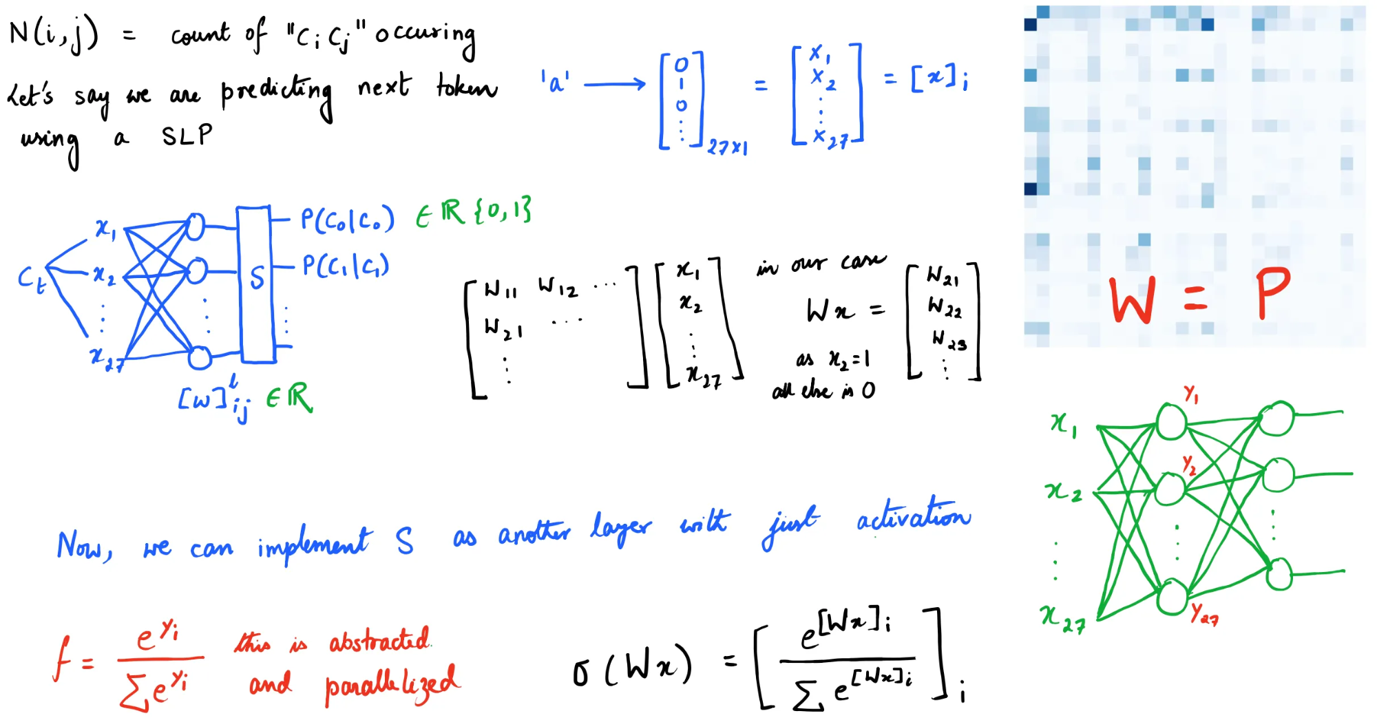
Note that this doesn’t include inferencing. What’s inferencing? Well in this case its generating the next token (character for us).

Code for training.

"""Training"""

# Setup
xs, ys = [], []
for w in words:
    w = '.' + w + '.'
    for ch1, ch2 in zip(w, w[1:]):
        ch1_idx = stoi[ch1]
        ch2_idx = stoi[ch2]
        xs.append(ch1_idx)
        ys.append(ch2_idx)
xs = torch.tensor(xs)
ys = torch.tensor(ys)
num = xs.nelement()

# Initialize random weights
W = torch.randn((27, 27), generator=torch.Generator(), requires_grad=True)

for k in range(100):
    # Forward Pass
    xenc = F.one_hot(xs, num_classes=27).float()
    logits = xenc @ W
    # The following is basically softmax.
    counts = logits.exp()
    probs = counts / counts.sum(1, keepdims=True)
    loss = -probs[torch.arange(num), ys].log().mean()

    # Backward Pass
    W.grad = None
    loss.backward()

    # Update
    W.data += -0.05 * W.grad

Code for inferencing.

"""Inferencing"""

ix = 0
name = ""
while True:
    xenc = F.one_hot(torch.tensor([ix]), num_classes=27).float()
    logits = xenc @ W
    probs = F.softmax(logits, dim=1)
    ix = torch.multinomial(probs, num_samples=1).item()
    if ix == 0:
        break
    name += itos[ix]
print(name)

Inference setup is almost always different from training and in our case it will be something like the following.

Regularization¶

Regularization is any technique that trades “perfect” training accuracy for better generalization.

Why regularization?

smooth (simple) weight distribution
making model less confident or extreme to avoid overfitting
programming humility and simplicity
occam's razor and generalization

How do we do it? Let’s see an example.

Original loss or just negative log likelihood,

\[ \mathcal{L} = -\frac{1}{n}\sum_{i=1}^{n} \log P(y_i|x_i) \]

and with gravitational force (L2 regularization),

\[ \mathcal{L}_{reg} = -\frac{1}{n}\sum_{i=1}^{n} \log P(y_i|x_i) + \lambda \sum_{i,j} W_{i,j}^2 \]

with that \(\lambda \sum W^2\) term as gravity - it constantly pulls all weights toward zero. The bigger the weights get, the stronger the pull back.

How does this lead to smoothness? The L2 term in loss function pushes for a flat probability distribution. Smoothness technically behaves like is an implicit prior bias that values simplicity and generalization.

MLP¶

[TODO]

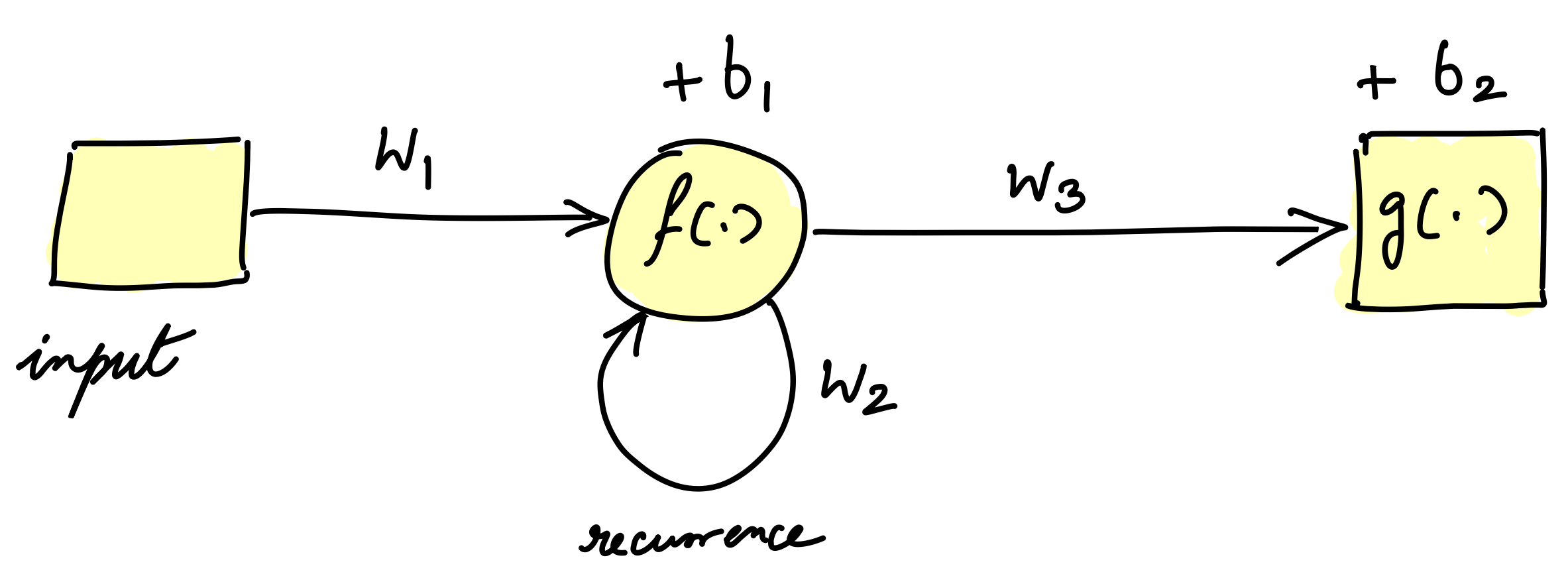
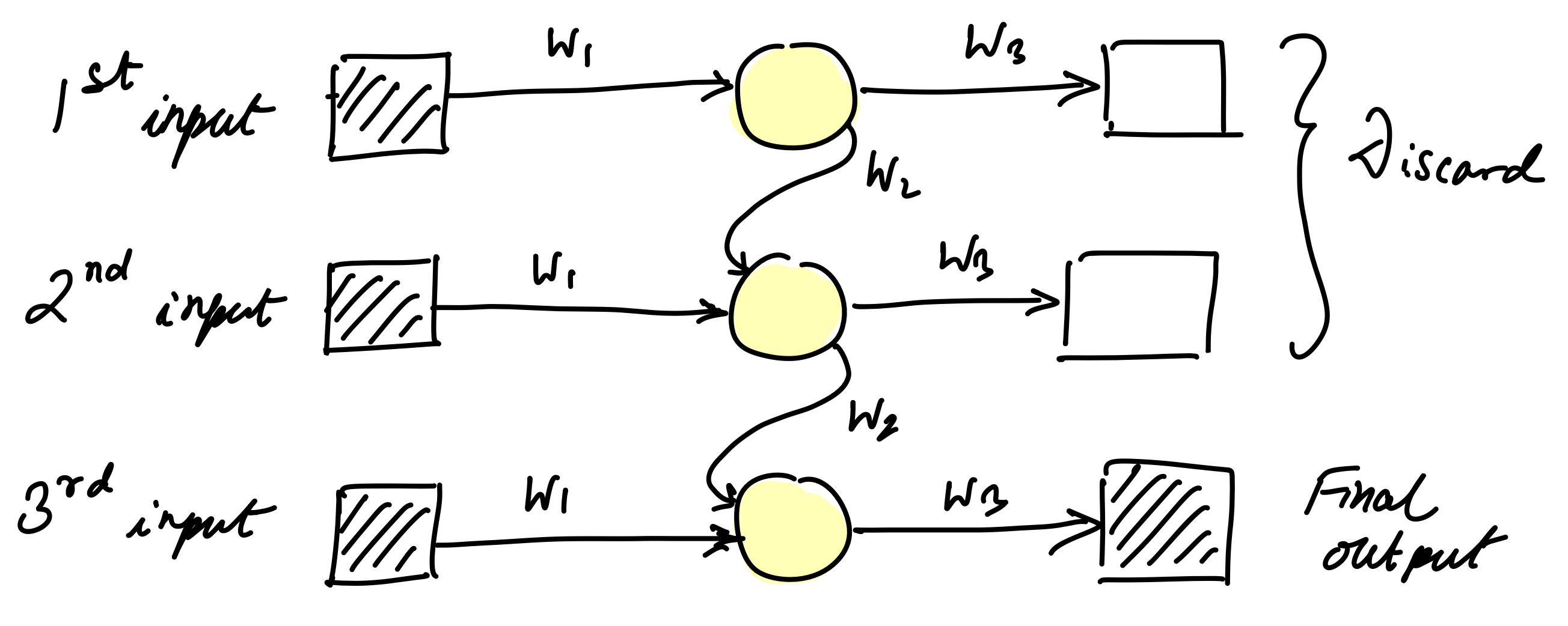
RNN¶

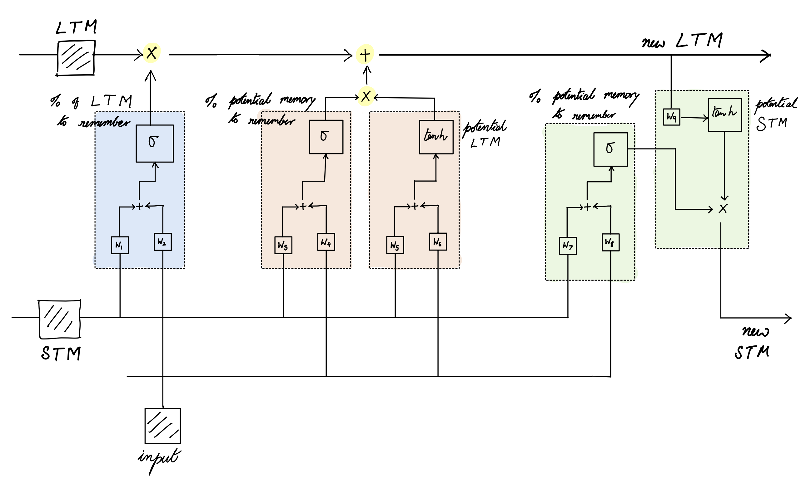
LSTM¶

Transformers¶

[TODO]

Walls before LLMs¶

Single layer perceptrons can only solve linearly separable problems.
- Cannot learn XOR function or overlapping patterns etc.
- Breakthrough: training multiple layers is possible with backpropagation.
- SOTA: universal approximation theorem.
Shallow networks worked well. But deep networks couldn’t train because gradients disappeared in early layers.
- Traditional activation functions (sigmoid and tanh) have very small derivatives in the flat parts of their S-shape.
- Breakthrough: layer wise pre-training.
- SOTA: ReLU (better activation functions), normalization, skip connections (ResNet), better weight initialization (Xavier).
Standard MLPs can only handle fixed-size inputs, but language has variable-length sequences.
- Cannot process sentences of different lengths.
- No memory of previous words in a sequence.
- Had to truncate or pad all inputs to same length.
- Breakthrough: Recurrent Neural Networks (RNNs) with recurrent connections that maintain hidden state.
RNNs couldn't learn long-term dependencies - gradients vanish over long sequences.
- Same vanishing gradient problem as deep networks, but across time steps.
- Models forgot information from early in the sequence.
- Couldn't learn relationships between distant words.
- Breakthrough: LSTM (1997) and GRU (2014) with gating mechanisms that control information flow. Gradient clipping.
RNNs / LSTMs process sequences one step at a time, making training extremely slow.
- Cannot parallelize across sequence length.
- Training time scales linearly with sequence length.
- GPU utilization was poor due to sequential dependencies.
- Breakthrough: Attention mechanisms (2015) allowing direct connections between all positions.
Seq2seq models created an information bottleneck at the encoder-decoder boundary.
- Entire input sequence compressed into single fixed-size context vector.
- Decoder has no direct access to input tokens, only final encoder state.
- Performance degrades severely with longer input sequences.
- Context vector becomes a lossy compression of all input information.
- Breakthrough: Attention mechanisms (2015) allowing decoder to directly attend to encoder states.
Early attention mechanisms still relied on RNN / LSTM backbone architectures.
- Attention was just an add-on to sequential RNN processing.
- Still couldn't parallelize the core sequence processing.
- Complex alignment and attention weight computation.
- Required separate encoder and decoder RNN stacks.
- Breakthrough: Pure attention architecture (Transformer 2017) eliminating recurrence entirely.
Encoder-decoder training inefficiencies for language modeling.
- Required separate encoder and decoder stacks (doubled model size).
- Cross-attention between encoder and decoder added complexity.
- Bidirectional encoder couldn't be used for autoregressive generation.
- Training required paired input-output data.
- Breakthrough: Decoder-only architecture (GPT) using pure autoregressive self-attention.

Large Language Models¶

[TODO: type out my notes on RNN, LSTM, Neural Turing Machine and Attention]

[TODO: finish reading the Transformer Family article]

Tokens and Thoughts¶

[TODO: type out my notes from the 2 papers]

Philosophy¶

[TODO: finish reading rest of the paper and then type out my notes from the paper]

References¶

Philosophy of Language by Martinich
Understanding Deep Learning by Prince
Attention? Attention! by Lilian Weng
The Transformer Family Version 2.0 by Lilian Weng
Driven by Compression Progress by Schmidhuber
From Tokens to Thoughts by LeCun and others
A Philosophical Introduction to Language Models by Milliere and Buckner
On the Measure of Intelligence (ARC Paper) by Francois Chollet
Large Language Models and Linguistic Intentionality by Jumbly Grindrod
Searching Latent Program Spaces by Clement Bonnet and others
Combining Induction and Transduction by Kevin Ellis and others
Godel Disjunction by Wrigley
On Paraconsistent Logic
Four sons of Penrose by Dershowitz
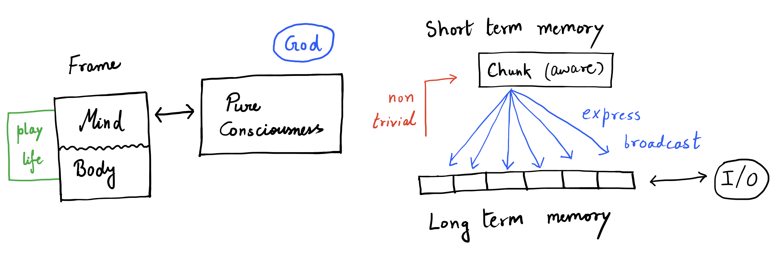
Brainish by Paul Liang
Conscious Turing Machines by Manuel and Lenore Blum
Minds, Machines, and Mathematics by David Chalmers